Earlier in these notes I used the Rescorla-Wagner model of associative learning as an example of how to implement computational models of cognition in R. In this and later sections, I’ll expand the dicussion of models to cover a variety of other models in the field. I’ll start with the backpropagation rule for learning in connectionist networks.
1 Scripts and data set
The iris_recode.csv file contains the classic iris data slightly reorganised as purely numeric data (here) is the script that generated it.
The first version of the modelling code implements a simple two-layer backpropagation network for the iris data: iris_twolayer.R
The second version of the code implements the same model, but expressing the learning rules as matrix operations in order to speed up the calculations: iris_twolayer2.R
At the moment the scripts don’t do anything other than learn a classification rule. The goal for the full exercise will (eventually) be to examine what the model is learning across the series of “epochs”, and consider the relationship between this connectionist network and a probabilistic logistic regression model, but for now it’s a bit simpler than that!
In this tutorial we’ll only cover a very simple version of a backpropagation network, the two-layer “perceptron” model. There are two versions of the code posted above. The code in the iris_twolayer.R script is probably the more intuitive version, as it updates the association weights one at a time, but R code runs much faster when you express the learning rule using matrix operations, which is hwat the iris_twolayer2.R version does. Let’s start with a walk through of the more intuitive version…
2 Input and output patterns
First, let’s take a look at the training data. I’m going to use the classic “iris” data set that comes bundled with R, but I’ve reorganised the data in a form that is a little bit more useful for thinking about the learning problem involved, and expressed it as a numeric matrix.
Rows: 150 Columns: 8
── Column specification ────────────────────────────────────────────────────────
Delimiter: ","
dbl (8): sepal_length, sepal_width, petal_length, petal_width, context, spec...

ℹ Use `spec()` to retrieve the full column specification for this data.
ℹ Specify the column types or set `show_col_types = FALSE` to quiet this message.
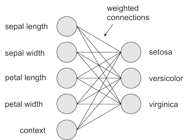
This data set has columns containing many features. First there are the input features, which consist of two features relating to the petals, two features relating to the sepal, and a context feature that is 1 for every flower. Additionally, there are three binary valued output features corresponding to the species of each flower, dummy coded so that only the correct species has value 1 and the incorrect species have value 0. Here are the names:
In its simplest form we can describe the knowledge possessed by our network as a set of associative strengths between every input feature and every output feature. In that sense we can think of it as a generalisation of how the Rescorla-Wagner model represents knowledge:
So what we’ll do is create a weight matrix that sets the initial associative strength to zero, with a tiny bit of random noise added to each of these associative weights:
In the Rescorla-Wagner model, when the learner is shown a compound stimulus with elements A and B with individual associative strengths \(v_A\) and \(v_B\), the association strength for the compound AB is assumed to be additive \(v_{AB} = v_{A} + v_{B}\). We could do this for our backpropagation network too, but it is much more common to assume a logistic activation function. So we’ll need to define this activation function:
logit <-function(x){ y <-1/(1+exp(-x))return(y)}
So what we do is first take the sum of the inputs and then pass them through our new logit function. So let’s say we want to compute the strength associated with the first species:
More generally though we can loop over the three species:
# initialise the output nodes at zerooutput <-rep(0, n_output)names(output) <- output_names# feed forward to every output node by taking a weighted sum of# the inputs and passing it through a logit functionfor(o in1:n_output) { output[o] <-sum(input * weight[,o]) %>%logit() }# print the resultoutput
Here is the code implementing the learning rule. What we’re doing is looping over every weight in the network, and then adjusting the strength proportional to the prediction error:
learning_rate <- .1# for each of the weights connecting to an output node...for(o in1:n_output) {for(i in1:n_input) {# associative learning for this weight scales in a manner that depends on# both the input value and output value. this is similar to the way that# Rescorla-Wagner has CS scaling (alpha) and US scaling (beta) parameters# but the specifics are slightly different (Equation 5 & 6 in the paper) scale_io <- input[i] * output[o] * (1-output[o]) # adjust the weights proportional to the error and the scaling (Equation 8) weight[i,o] <- weight[i,o] + (prediction_error[o] * scale_io * learning_rate) }}
(Let’s not worry too much about the scale_io factor for now). So let’s look at the input, output, target, and prediction error:
Not surprisingly everything to setosa has gone up and the others down. But notice the scale!
6 Visualising the learning
For the actual simulation I’ll set the learning rate to .01, run it for 5000 epochs and average across 100 independent runs just to smooth out any artifacts of randomisation1 How the weights change over epochs:
Footnotes
The script to run it is here, a csv with the connections weights is here, another one (36Mb) with sum squared error to each item on each presentation here, zipped version (11Mb) here↩︎