Thou shalt not answer questionnaires Or quizzes upon World Affairs, Nor with compliance Take any test. Thou shalt not sit With statisticians nor commit A social science
load("./data/afl24.Rdata") # load datahead(afl) # show the first few rows
         home.team away.team home.score away.score year round weekday day month
1  North Melbourne  Brisbane        104        137 1987     1     Fri  27     3
2 Western Bulldogs  Essendon         62        121 1987     1     Sat  28     3
3          Carlton  Hawthorn        104        149 1987     1     Sat  28     3
4      Collingwood    Sydney         74        165 1987     1     Sat  28     3
5        Melbourne   Fitzroy        128         89 1987     1     Sat  28     3
6         St Kilda   Geelong        101        102 1987     1     Sat  28     3
  is.final              venue attendance
1    FALSE                MCG      14096
2    FALSE      Waverley Park      22550
3    FALSE       Princes Park      19967
4    FALSE      Victoria Park      17129
5    FALSE                MCG      18012
6    FALSE Gold Coast Stadium      15867
1 Confidence intervals
As usual there are many ways to compute the confidence interval of the mean in R. One relatively simple one is with the ciMean function in the lsr package, which (conveniently) can take a data frame as input and computes confidence intervals for all the numeric variables:
ciMean(afl)
                   2.5%       97.5%
home.team*           NA          NA
away.team*           NA          NA
home.score   100.621214   102.39555
away.score    90.250700    91.98720
year        1998.566873  1998.97782
round         11.999916    12.40185
weekday*             NA          NA
day           15.594242    16.13388
month          6.006252     6.10548
is.final*            NA          NA
venue*               NA          NA
attendance 31597.324710 32593.12361
By default it returns a 95% confidence interval, but you can adjust the conf argument if you want something different. For instance, here’s an 80% confidence interval
ciMean(x = afl, conf = .8)
                    10%          90%
home.team*           NA           NA
away.team*           NA           NA
home.score   100.928367   102.088392
away.score    90.551304    91.686592
year        1998.638012  1998.906681
round         12.069495    12.332274
weekday*             NA           NA
day           15.687658    16.040461
month          6.023429     6.088303
is.final*            NA           NA
venue*               NA           NA
attendance 31769.706887 32420.741437
You can also give it a single variable as input if you like:
ciMean( afl$home.score )
         2.5%    97.5%
[1,] 100.6212 102.3955
2 Comparing two means
Does the home team tend to outscore the away team? This requires a paired samples t-test:
   Paired samples t-test

Variables:  home.score , away.score

Descriptive statistics:
            home.score away.score difference
   mean        101.508     91.119     10.389
   std dev.     29.660     29.027     44.335

Hypotheses:
   null:        population means equal for both measurements
   alternative: different population means for each measurement

Test results:
   t-statistic:  15.359
   degrees of freedom:  4295
   p-value:  <.001

Other information:
   two-sided 95% confidence interval:  [9.063, 11.716]
   estimated effect size (Cohen's d):  0.234
Are finals games lower scoring than home and away games? This requires an independent samples t-test:
Warning in independentSamplesTTest(total.score ~ is.final, afl): group variable
is not a factor
   Welch's independent samples t-test

Outcome variable:   total.score
Grouping variable:  is.final

Descriptive statistics:
              FALSE    TRUE
   mean     193.064 183.680
   std dev.  38.602  34.235

Hypotheses:
   null:        population means equal for both groups
   alternative: different population means in each group

Test results:
   t-statistic:  3.762
   degrees of freedom:  224.433
   p-value:  <.001

Other information:
   two-sided 95% confidence interval:  [4.468, 14.3]
   estimated effect size (Cohen's d):  0.257
3 Categorical associations
Are all teams equally likely to play their home games on every weekday? For that we might consider using a chi-square test of categorical association, but as you can see from the output below, a little care is needed:
The reason for the warning, of course, is that with so few games played on weekdays, many of the expected cell counts are very small, and that violates one of the assumptions of the chi-square test. So let’s create a new variable that collapses these:
Now we just have three levels of this factor, corresponding to Saturday games, Sunday games, and weekday games. So if we run the test of association with this version of the variable we no longer get the warning message:
associationTest(~ home.team + weekday_small, afl)
     Chi-square test of categorical association

Variables:   home.team, weekday_small

Hypotheses:
   null:        variables are independent of one another
   alternative: some contingency exists between variables

Observed contingency table:
                  weekday_small
home.team          M-F Sat Sun
  Adelaide          27  94 114
  Brisbane          19 132 131
  Carlton           25 179  62
  Collingwood       64 167  55
  Essendon          65 158  66
  Fitzroy            6  84  10
  Fremantle         21  66  92
  Geelong           21 185  79
  Hawthorn          27 189  63
  Melbourne         51 140  87
  North Melbourne   93 123  69
  Port Adelaide     17  78  69
  Richmond          61 138  68
  St Kilda          37 174  68
  Sydney            31  85 161
  West Coast        53  93 138
  Western Bulldogs  31 141  89

Expected contingency table under the null hypothesis:
                  weekday_small
home.team           M-F   Sat  Sun
  Adelaide         35.5 121.8 77.7
  Brisbane         42.6 146.1 93.3
  Carlton          40.2 137.8 88.0
  Collingwood      43.2 148.2 94.6
  Essendon         43.7 149.7 95.6
  Fitzroy          15.1  51.8 33.1
  Fremantle        27.0  92.8 59.2
  Geelong          43.1 147.7 94.3
  Hawthorn         42.1 144.6 92.3
  Melbourne        42.0 144.0 92.0
  North Melbourne  43.1 147.7 94.3
  Port Adelaide    24.8  85.0 54.2
  Richmond         40.3 138.3 88.3
  St Kilda         42.1 144.6 92.3
  Sydney           41.8 143.5 91.6
  West Coast       42.9 147.2 93.9
  Western Bulldogs 39.4 135.2 86.3

Test results:
   X-squared statistic:  480.877
   degrees of freedom:  32
   p-value:  <.001

Other information:
   estimated effect size (Cramer's v):  0.237
4 Comparing several means
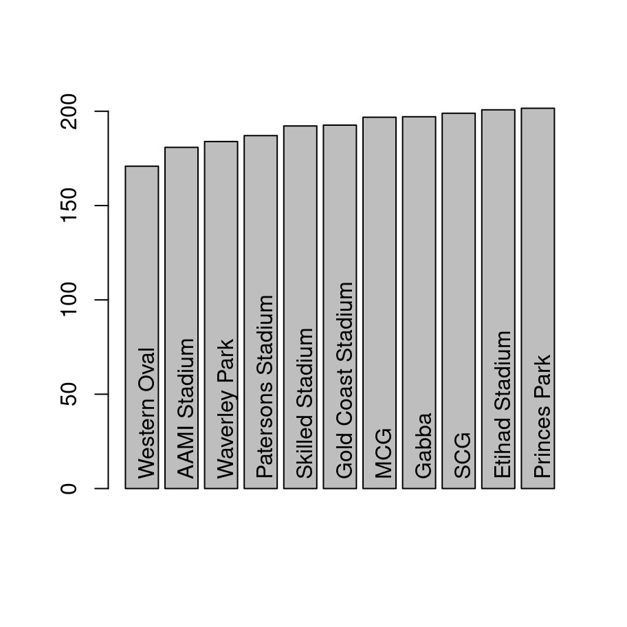
Is there such a thing as a “high scoring ground”? Let’s take a look at the average number of points per game at each different ground, only considering grounds that had at least 100 games played during the the time period:
venue.use <-table(afl$venue)majors <- venue.use[venue.use >=100]# restrict the data to these gamesafl.majors <- afl[ afl$venue %in%names(majors), ]
Visually it does look like there might something here:
A first pass analysis for this would be ANOVA. The underlying statistical model in ANOVA and multiple regression is essentially the same, and the work is done by the lm function in R. However, it’s generally considered sensible to use the aov function in the first instance, because that does a few nice things that come in handy with later analyses.
mod <-aov(total.score ~ venue, afl.majors)
To analyse it as an ANOVA, the Anova function in the car package is very nice:
Anova(mod)
Anova Table (Type II tests)

Response: total.score
           Sum Sq   Df F value    Pr(>F)
venue      237330   10  16.616 < 2.2e-16 ***
Residuals 5681696 3978
---
Signif. codes:  0 '***' 0.001 '**' 0.01 '*' 0.05 '.' 0.1 ' ' 1
It seems to be a real thing, but we’ll come back to that in a moment because we might have some worries about confounding variables.
4.1 Post hoc tests
I am not a fan of post hoc tests, even with corrections for Type I error inflation. To see why they drive me nuts, let’s run the output of the ANOVA through the posthocPairwiseT function. By default it uses the Holm correction, but lets just use the simpler and very conservatice Bonferroni correction:
    Pairwise comparisons using t tests with pooled SD

data:  total.score and venue

                   AAMI Stadium Etihad Stadium Gabba   Gold Coast Stadium
Etihad Stadium     3.1e-13      -              -       -
Gabba              2.0e-05      1.00000        -       -
Gold Coast Stadium 0.20642      1.00000        1.00000 -
MCG                3.8e-11      1.00000        1.00000 1.00000
Patersons Stadium  1.00000      5.0e-06        0.09684 1.00000
Princes Park       2.7e-11      1.00000        1.00000 1.00000
SCG                1.6e-07      1.00000        1.00000 1.00000
Skilled Stadium    0.02836      0.34402        1.00000 1.00000
Waverley Park      1.00000      1.1e-08        0.00317 1.00000
Western Oval       0.75909      2.4e-12        1.4e-07 0.00096
                   MCG     Patersons Stadium Princes Park SCG
Etihad Stadium     -       -                 -            -
Gabba              -       -                 -            -
Gold Coast Stadium -       -                 -            -
MCG                -       -                 -            -
Patersons Stadium  0.00075 -                 -            -
Princes Park       1.00000 2.6e-05           -            -
SCG                1.00000 0.00573           1.00000      -
Skilled Stadium    1.00000 1.00000           0.31433      1.00000
Waverley Park      2.0e-06 1.00000           1.3e-07      9.0e-05
Western Oval       2.7e-10 0.00371           9.9e-12      3.5e-09
                   Skilled Stadium Waverley Park
Etihad Stadium     -               -
Gabba              -               -
Gold Coast Stadium -               -
MCG                -               -
Patersons Stadium  -               -
Princes Park       -               -
SCG                -               -
Skilled Stadium    -               -
Waverley Park      0.74049         -
Western Oval       9.2e-05         0.08420

P value adjustment method: bonferroni
My main complaint? I have no idea what this means because I didn’t really have any idea what I was looking for. I could certainly run through all these automatically-detected “significant” relationships to see what makes any sense, but I honestly don’t know what that would buy me. Basically I’m not sure why I’m calculating a \(p\)-value (a tool designed to test hypotheses) in a situation where I really didn’t have any hypotheses ahead of time. To my mind this use of hypothesis testing has the effect of eroding the boundary between confirmatory tests (where the researcher has a theory ahead of time), and exploratory analyses (where we’re just looking for interesting patterns). I’m a big fan of doing both things as part of science, of course, I just think they need to be kept clearly separate :-)
But that’s a topic for another time.
5 Assessing relationships
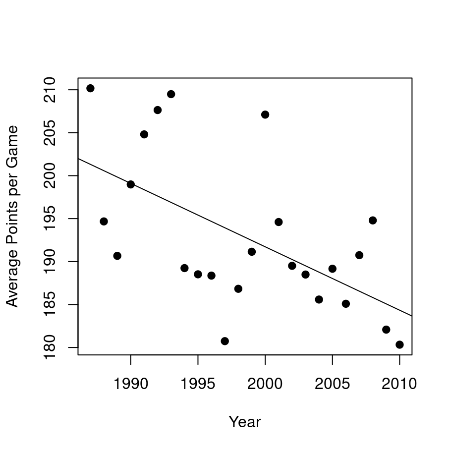
One thing that people commented on a lot during this time period was the fact that the games became lower scoring over time. Is that a real effect, or was it just random noise?
mod <-lm(total.score ~ year, afl)summary(mod)
Call:
lm(formula = total.score ~ year, data = afl)

Residuals:
    Min      1Q  Median      3Q     Max
-148.84  -24.20   -0.09   24.71  139.02

Coefficients:
              Estimate Std. Error t value Pr(>|t|)
(Intercept) 1668.10138  169.27250   9.855   <2e-16 ***
year          -0.73819    0.08469  -8.717   <2e-16 ***
---
Signif. codes:  0 '***' 0.001 '**' 0.01 '*' 0.05 '.' 0.1 ' ' 1

Residual standard error: 38.13 on 4294 degrees of freedom
Multiple R-squared:  0.01739,   Adjusted R-squared:  0.01716
F-statistic: 75.98 on 1 and 4294 DF,  p-value: < 2.2e-16
yearly.score <-aggregate( total.score ~ year, data = afl, FUN = mean)plot(x = yearly.score$year,y = yearly.score$total.score,type ="p",pch =19,xlab ="Year",ylab ="Average Points per Game")abline(coef = mod$coef)
That’s pretty clearly a real effect, but it does open up a new line of worries about the last analysis…
5.1 Hierarchical regression
Suppose we’re a little paranoid. Maybe the effect of venue is spurious: some grounds came into use at different years, and we know there’s an effect of year on the total.score. Similarly, folk wisdom has it that finals games are lower scoring, and those games are disproportionately likely to be played at the MCG. Maybe there’s an effect of the size of the crowd? Some stadiums are bigger than others? Maybe there’s an effect of weekday, and some venues do indeed get used on different days. Maybe it’s an effect of the teams playing, since different teams tend to play at different grounds (especially when considering the home team!) To address this let’s dump all those variables into a regression model, and then see if adding venue leads to an improvement in fit over and above those. In other words, we’ll do a hierarchical regression. Here it is in R:
Analysis of Variance Table

Model 1: total.score ~ year + home.team + away.team + is.final + weekday +
    attendance + venue
Model 2: total.score ~ year + home.team + away.team + is.final + weekday +
    attendance
  Res.Df     RSS  Df Sum of Sq      F    Pr(>F)
1   3937 5266076
2   3947 5519332 -10   -253256 18.934 < 2.2e-16 ***
---
Signif. codes:  0 '***' 0.001 '**' 0.01 '*' 0.05 '.' 0.1 ' ' 1
Overall it does rather look like there are genuine differences between venues. Though of course there could be many other things we didn’t control for!
5.2 Testing a correlation
As an aside, it’s often noted that a Pearson correlation is essentially equivalent to a linear regression model with a single predictor. So we should be able to replicate the total.score ~ year analysis as a correlation. We use the cor.test function to run a hypothesis test here:
cor.test(x = afl$total.score, y = afl$year)
    Pearson's product-moment correlation

data:  afl$total.score and afl$year
t = -8.7166, df = 4294, p-value < 2.2e-16
alternative hypothesis: true correlation is not equal to 0
95 percent confidence interval:
 -0.1611277 -0.1023575
sample estimates:
       cor
-0.1318585
To see that these are giving the same answer, let’s take the raw correlation of \(r=-.13\), square it, and compare it to the (unadjusted) \(R^2\) value of 0.01739 reported above: